Using XLOOKUP with Multiple Lookup Values in Excel: How-to Guide

Pierceli

Editor

posted on 8 months ago — updated on 1 second ago

65
views

XLOOKUP is a handy Excel function, but what if you want to find some data in your spreadsheet that requires multiple search criteria to find? When you look at the XLOOKUP formula, it appears that you can only add one lookup value. However, you can get around this by using Boolean logic or concatenation to instruct XLOOKUP to use multiple search criteria. Keep reading to learn more.

The Basics of Using XLOOKUP with Multiple Criteria

Multiple Criteria with Boolean Logic

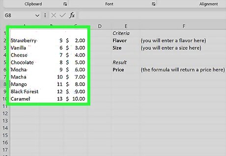
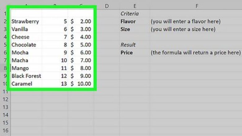
Understand how Boolean logic works with the formula. Normally, XLOOKUP can only look for one value. However, you can use Boolean logic in the XLOOKUP formula, which creates a temporary lookup array of 1's (TRUE) and 0's (FALSE) to return a result that matches all of the lookup criteria. Example: You have a spreadsheet with columns for cake flavors, cake sizes, and prices. You want to create an XLOOKUP formula with Boolean logic that will look up the price of a cake based on the flavor and size that you input. The basic XLOOKUP formula using Boolean logic to look up multiple criteria looks like this: =XLOOKUP(1, (lookup_array1=lookup_value1) * (lookup_array2=lookup_value2) * (insert one array for each lookup_value), return_array)

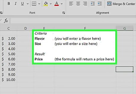
Create "Criteria" and "Result" sections in your spreadsheet. The "Criteria" section will be used to input lookup values into your formula, and the "Result" section is where you will actually put your XLOOKUP formula to get the intended result. Example: Your spreadsheet has 3 columns (cake flavors, cake sizes, and prices) that are in columns A, B, and C. Skip column D, then put the "Criteria" and "Result" sections in columns E and F as follows: E F 1 Criteria 2 Flavor (you will enter a flavor here) 3 Size (you will enter a size here) 4 5 Result 6 Price (the formula will return a price here)

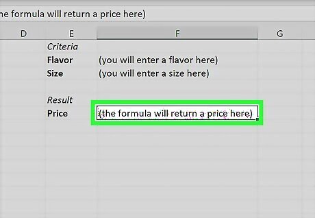
Select the cell to the right of the labeled cell in the "Result" section. This cell is where you'll enter the XLOOKUP formula. Example: In the example, the cell labeled Price in the "Result" section is E6, so you should select F6 (one cell to the right).

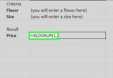
Type =XLOOKUP(1, in the cell. Comparing this to the basic XLOOKUP formula (=XLOOKUP(lookup_value, lookup_array, result_array)), the 1 in the XLOOKUP Boolean logic formula is considered the lookup_value. The reason that you set 1 as the lookup_value is because "1" correlates to "TRUE." When you input lookup criteria into your formula, XLOOKUP will check that criteria against the arrays in the formula and create an array of TRUE and FALSE values. These values are then converted into numbers, and XLOOKUP will then look for the first 1 in that array (in other words, the first result that matches all of the lookup criteria).

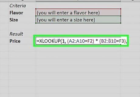
Add your lookup criteria with Boolean logic. For each lookup criteria, you should have a matching lookup array. These pairs should be written like (lookup_array)=(lookup_value). Separate each pair with an asterisk (*), and add a comma after the last array/value set. Your lookup array will be the cell range that contains the information you want to look through for that particular lookup value. Your lookup value will reference one of the cells under the "Criteria" section you made in Step 2. Example: Your lookup arrays will be the contents of the "flavor" and "size" columns. Each column has 9 rows of data, so the flavor array is A2:A10 and the size array is B2:B10. Your lookup values will be F2 (for flavor) and F3 (for size) as they are the cells directly to the right of the Flavor and Size labels in the "Criteria" section. With this information, you can add the array/value sets to your formula, which looks like this so far: =XLOOKUP(1, (A2:A10=F2) * (B2:B10=F3),

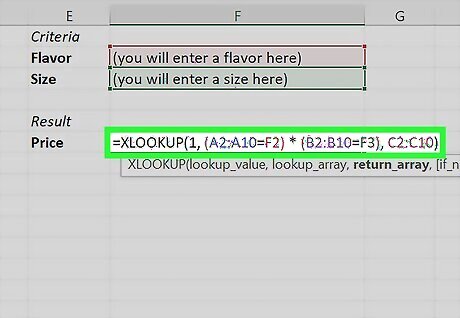
Add your results array. This is the range of cells that you want to get your results from. After adding your results array to the formula, add a ) to finish the formula. Example: You want to get your results from the "price" column, so your results array is C2:C10. Your finished formula with the results array looks like this: =XLOOKUP(1, (A2:A10=F2) * (B2:B10=F3), C2:C10)

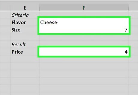
Test your formula by entering some lookup values in the "Criteria" section. In the example, you would enter a cake flavor in F2 and a cake size in F3, and the formula should return the corresponding price for that combination in F6. If your formula is not returning the right result or it's giving you an error, double check that all of the cell references in your formula are correct. Excel color codes cell references in formulas when you're editing them, so you can easily see if one of your references is incorrect.

Multiple Criteria with Concatenation

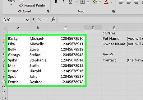
Understand what concatenation does in the formula. Concatenation uses the & operator to join values together. Using concatenation, you can get around the XLOOKUP formula only accepting one lookup value by combining the two values together. Example: You have a spreadsheet with columns for pet names, pet owners, and contact information. You want to create an XLOOKUP formula with with concatenation that looks up a pet owner's contact information if you input the name of them and their pet. The basic XLOOKUP formula using concatenation to look up multiple criteria looks like this: =XLOOKUP(lookup_value1 & lookup_value2 & [insert each lookup value], lookup_array1 & lookup_array2 & [insert each lookup array], return_array)

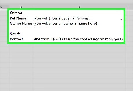
Create "Criteria" and "Result" sections in your spreadsheet. The "Criteria" section will be used to input lookup values into your formula, and the "Result" section is where you will actually put your XLOOKUP formula to get the intended result. Example: Your spreadsheet has 3 columns (pet names, owner's names, and contact information) that are in columns A, B, and C. Skip column D, then put the "Criteria" and "Result" sections in columns E and F as follows: E F 1 Criteria 2 Pet Name (you will enter a pet's name here) 3 Owner Name (you will enter an owner's name here) 4 5 Result 6 Contact (the formula will return the contact information here)

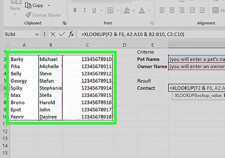
Determine what information you need for each argument. In an XLOOKUP formula, you have three arguments: a lookup_value, a lookup_array, and a return_array. When you're using concatenation, the lookup_value and lookup_array will be concatenated by putting & between each value or array. The lookup_value will reference the cells next to your criteria labels in the "Criteria" section you made in step 2. The lookup_array will reference the cell ranges that contain the lookup criteria. The return_array will be one range of cells that you are getting your result from. Example: In your spreadsheet, your lookup values are cells F2 (for pet name) and F3 (for owner name). You have 9 rows of data in your spreadsheet (rows 2 through 10) and your lookup criteria is referencing information from columns A and B. Column C is where you are getting your results from. You determine that your lookup value is F2 & F3, your lookup array is A2:A10 & B2:B10, and your return array is C2:C10.

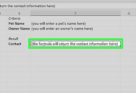
Select the cell to the right of the labeled cell in the "Result" section. This cell is where you'll enter the XLOOKUP formula. Example: In the example, the cell labeled Contact in the "Result" section is E6, so you should select F6 (one cell to the right).

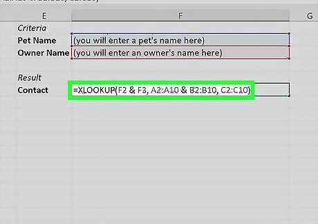
Write an XLOOKUP formula using your concatenated strings. Take the information you determined in Step 3 and combine them into an XLOOKUP formula. In the example, your XLOOKUP formula would look like this: =XLOOKUP(F2 & F3, A2:A10 & B2:B10, C2:C10)

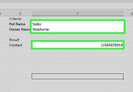
Test your formula by entering some lookup values in the "Criteria" section. In the example, you would enter a pet name in F2 and an owner name in F3, and the formula should return the corresponding contact information for that combination in F6. If your formula is not returning the right result or it's giving you an error, double check that all of the cell references in your formula are correct. Excel color codes cell references in formulas when you're editing them, so you can easily see if one of your references is incorrect.