views
Creating a Basic Spreadsheet

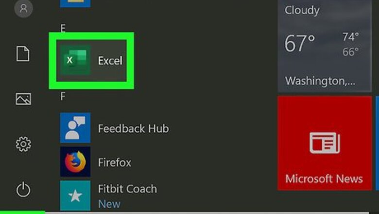
Open Microsoft Excel. You'll find it in the Start menu (Windows) or in the Applications folder (macOS). The app will open to a screen that allows you to create or select a document. If you don't have a paid version of Microsoft Office, you can use the free online version at https://www.office.com to create a basic spreadsheet. You'll just need to sign in with your Microsoft account and click Excel in the row of icons.
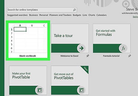
Click Blank workbook to create a new workbook. A workbook is the name of the document that contains your spreadsheet(s). This creates a blank spreadsheet called Sheet1, which you'll see on the tab at the bottom of the sheet. When you make more complex spreadsheets, you can add another sheet by clicking + next to the first sheet. Use the bottom tabs to switch between spreadsheets.
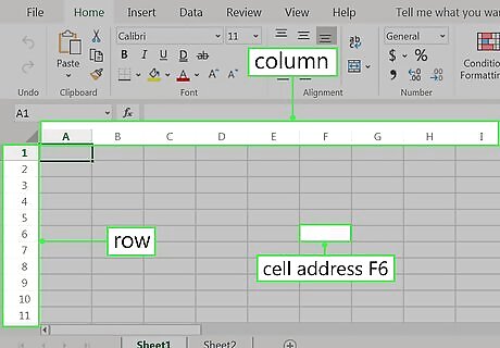
Familiarize yourself with the spreadsheet's layout. The first thing you'll notice is that the spreadsheet contains hundreds of rectangular cells organized into vertical columns and horizontal rows. Some important things to note about this layout: All rows are labeled with numbers along the side of the spreadsheet, while the columns are labeled with letters along the top. Each cell has an address consisting of the column letter followed by the row number. For example, the address of the cell in the first column (A), first row (1) is A1. The address of the cell in column B row 3 is B3.
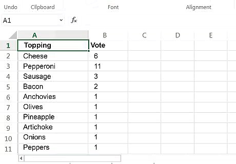
Enter some data. Click any cell one time and start typing immediately. When you're finished with that cell, press the Tab ↹ key to move to the next cell in the row, or the ↵ Enter key to the next cell in the column. Notice that as you type into the cell, the content also appears in the bar that runs across the top of the spreadsheet. This bar is called the Formula Bar and is useful for when entering long strings of data and/or formulas. To edit a cell that already has data, double-click it to bring back the cursor. Alternatively, you can click the cell once and make your changes in the formula bar. To delete the data from one cell, click the cell once, and then press Del. This returns the cell to a blank one without messing up the data in other rows or columns. To delete multiple cell values at once, press Ctrl (PC) or ⌘ Cmd (Mac) as you click each cell you want to delete, and then press Del. To add a new blank column between existing columns, right-click the letter above the column after where you'd like the new one to appear, and then click Insert on the context menu. To add a new blank row between existing rows, right-click the row number for the row after the desired location, and then click Insert on the menu.
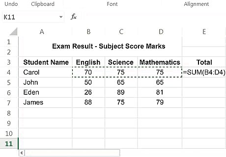
Check out the functions available for advanced uses. One of the most useful features of Excel is its ability to look up data and perform calculations based on mathematical formulas. Each formula you create contains an Excel function, which is the "action" you're performing. Formulas always begin with an equal (=) sign followed by the function name (e.g., =SUM, =LOOKUP, =SIN). After that, the parameters should be entered between a set of parentheses (). Follow these steps to get an idea of the type of functions you can use in Excel: Click the Formulas tab at the top of the screen. You'll notice several icons in the toolbar at the top of the application in the panel labeled "Function Library." Once you know how the different functions work, you can easily browse the library using those icons. Click the Insert Function icon, which also displays an fx. It should be the first icon on the bar. This opens the Insert Function panel, which allows you to search for what you want to do or browse by category. Select a category from the "Or select a category" menu. The default category is "Most Recently Used." For example, to see the math functions, you might select Math & Trig. Click any function in the "Select a function" panel to view its syntax, as well as a description of what the function does. For more info on a function, click the Help on this function. Click Cancel when you're done browsing. To learn more about entering formulas, see How to Type Formulas in Microsoft Excel.
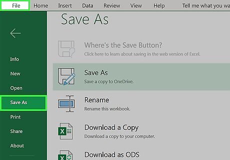
Save your file when you're finished editing. To save the file, click the File menu at the top-left corner, and then select Save As. Depending on your version of Excel, you'll usually have the option to save the file to your computer or OneDrive. Now that you've gotten the hang of the basics, check out the "Creating a Home Inventory from Scratch" method to see this information put into practice.
Creating a Home Inventory from Scratch
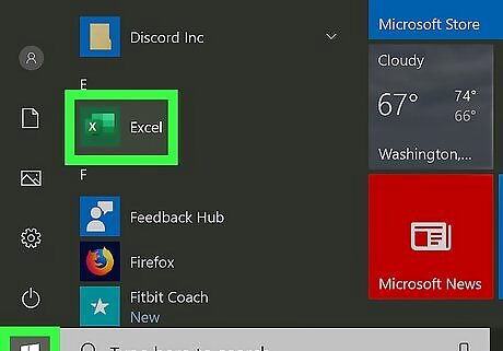
Open Microsoft Excel. You'll find it in the Start menu (Windows) or in the Applications folder (macOS). The app will open to a screen that allows you to create or open a workbook.
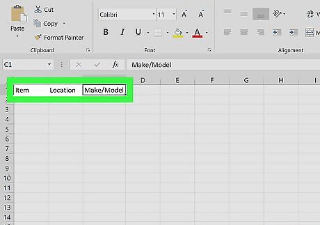
Name your columns. Let's say we're making a list of items in our home. In addition to listing what the item is, we might want to record which room it's in and its make/model. We'll reserve row 1 for column headers so our data is clearly labeled. Click cell A1 and type Item. We'll list each item in this column. Click cell B1 and type Location. This is where we'll enter which room the item is in. Click cell C1 and type Make/Model. We'll list the item's model and manufacturer in this column.
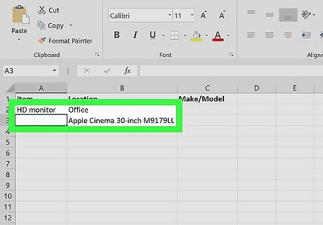
Enter your items on each row. Now that our columns are labeled, entering our data into the rows should be simple. Each item should get its own row, and each bit of information should get its own cell. For example, if you're listening the Apple HD monitor in your office, you may type HD monitor into A2 (in the Item column), Office into B2 (in the Location column), and Apple Cinema 30-inch M9179LL into B3 (the Make/Model column). List additional items on the rows below. If you need to delete a cell, just click it once and press Del. To remove an entire row or column, right-click the letter or number and select Delete. You've probably noticed that if you type too much text in a cell it'll overlap into the next column. You can fix this by resizing the columns to fit the text. Position the cursor on the line between the column letters (above row 1) so the cursor turns into two arrows, and then double-click that line.
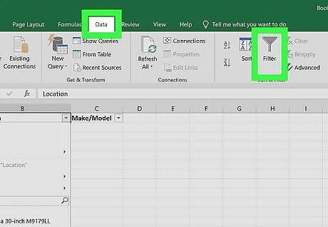
Turn the column headers into drop-down menus. Let's say you've listed hundreds of items throughout your home but only want to view those stored in your office. Click the 1 at the beginning of row 1 to select the whole row, and then do the following: Click the Data tab at the top of Excel. Click Filter (the funnel icon) in the toolbar. Small arrows now appear on each column header. Click the Location drop-down menu (in B1) to open the filter menu. Since we just want to see items in the office, check the box next to "Office" and remove the other checkmarks. Click OK. Now you'll only see items the selected room. You can do this with any column and any data type. To restore all items, click the menu again and check "Select All" and then OK to restore all items.
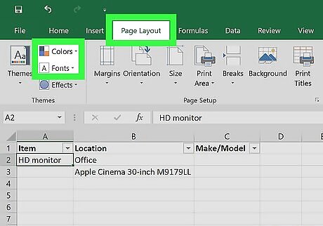
Click the Page Layout tab to customize the spreadsheet. Now that you've entered your data, you may want to customize the colors, fonts, and lines. Here are some ideas for doing so: Select the cells you want to format. You can select an entire row by clicking its number, or an whole column by clicking its letter. Hold Ctrl (PC) or Cmd (Mac) to select more than one column or row at a time. Click Colors in the "Themes" area of the toolbar to view and select color theme. Click the Fonts menu to browse for and select a font.

Save your document. When you've reached a good stopping point, you can save the spreadsheet by clicking the File menu at the top-left corner and selecting Save As.
Creating a Monthly Budget from a Template

Open Microsoft Excel. You'll find it in the Start menu (Windows) or in the Applications folder (macOS). The app will open to a screen that allows you to create or open a workbook. This method covers using a built-in Excel template to create a list of your expenses. There are hundreds of templates available for different types of spreadsheets. To see a list of all official templates, visit https://templates.office.com/en-us/templates-for-excel.
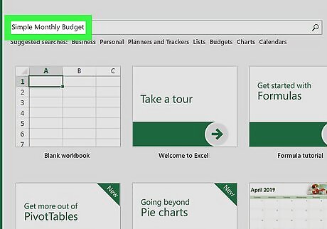
Search for the "Simple Monthly Budget" template. This is a free official Microsoft template that makes it easy to calculate your budget for the month. You can find it by typing Simple Monthly Budget into the search bar at the top and pressing ↵ Enter in most versions.
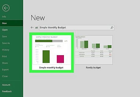
Select the Simple Monthly Budget template and click Create. This creates a new spreadsheet from a pre-formatted template. You may have to click Download instead.
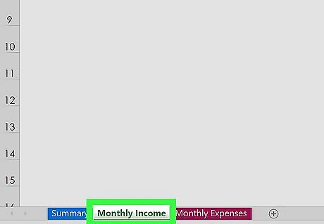
Click the Monthly Income tab to enter your income(s). You'll notice there are three tabs (Summary, Monthly Income, and Monthly Expenses) at the bottom of the workbook. You'll be clicking the second tab. Let's say you get income from two companies called wikiHow and Acme: Double-click the Income 1 cell to bring up the cursor. Erase the content of the cell and type wikiHow. Double-click the Income 2 cell, erase the contents, and type Acme. Enter your monthly income from wikiHow into the first cell under the "Amount" header (the one that says "2500" by default). Do the same with your monthly income from "Acme" in the cell just below. If you don't have any other income, you can click the other cells (for "Other" and "$250") and press Del to clear them. You can also add more income sources and amounts in the rows below those that already exist.
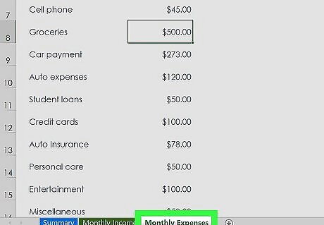
Click the Monthly Expenses tab to enter your expenses. It's the third tab at the bottom of the workbook. Those there are expenses and amounts already filled in, you can double-click any cell to change its value. For example, let's say your rent is $795/month. Double-click the pre-filled amount of "$800," erase it, and then type 795. Let’s say you don't have any student loan payments to make. You can just click the amount next to "Student Loans" in the "Amount" column ($50) and press Del on your keyboard to clear it. Do the same for all other expenses. You can delete an entire row by right-clicking the row number and selecting Delete. To insert a new row, right-click the row number below where you want it to appear, and then select Insert. Make sure there are no extra amounts that you don't actually have to pay in the "Amounts" column, as they'll be automatically factored into your budget.
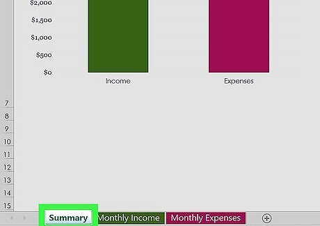
Click the Summary tab to visualize your budget. Once you've entered your data, the chart on this tab will automatically update to reflect your income vs. your expenses. If the info doesn't calculate automatically, press F9 on the keyboard. Any changes you make to the Monthly Income and Monthly Expenses tabs will affect what you see in your Summary.
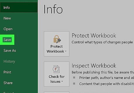
Save your document. When you've reached a good stopping point, you can save the spreadsheet by clicking the File menu at the top-left corner and selecting Save As.


Comments
0 comment